Modeling Non-sorted cicle ecosystems using the Water Ice and Temperature model (WIT)

WIT model

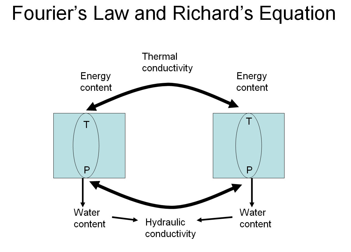
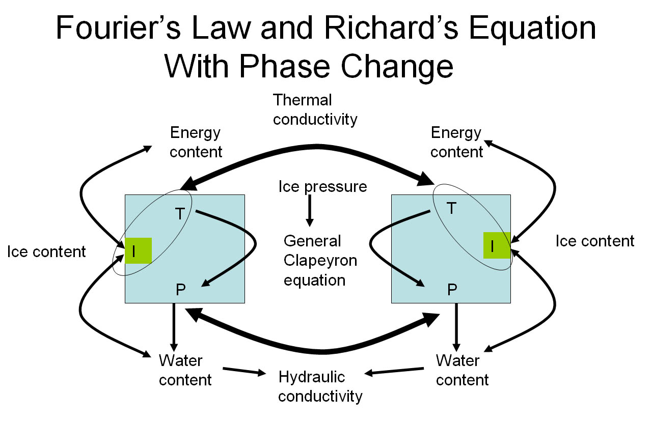
WIT is a coupled heat and moisture transfer model with phase change for a porous media. The model was developed for application in snow (Daanen and Nieber, 2009) and successfully applied in the non-sorted circle environment with comparison to field data (Daanen and Misra, 2008). The model simplifies the physical relationships governing the formation of ice in the active layer. The physical relations are simplified to the non-linear Richard equation for liquid water movement of variably saturated soils and Fourier's law for heat transfer with convection. Phase change is determined trough the General Calpeyron equation which shows the equilibrium conditions between the liquid water temperature, liquid water pressure and the ice pressure. When the soil conditions change the phase change will be corrected accordingly. When both liquid water and ice are present in the soil then the liquid water pressure, which determines liquid water flow, can be directly related to the temperature of the soil. The amount of ice formed in the soil is calculated through a constitutive relation between the liquid water pressure and the liquid water saturation of the soil, also known as the water retention curve. When e.g. the soil gets colder, below the freezing point, the liquid water pressure, or suction, becomes greater and the liquid water saturation becomes smaller. The change in saturation represents the change in ice content which results in a feedback to the temperature through latent heat release. This feedback is iterated till convergence exists. The result of this model is a three dimensional field of temperatures and ice contents in the freezing active layer.

Simplifications to the physics include the assumption that the ice pressure is zero at all times and all locations and that means that the rheology of the frozen soil is ignored. This also means that ice can accumulate in unlimited amounts wherever it is cold enough and water supply is sufficient. This also means that frost heave is not a variable in the model.

The freezing characteristic curve is often used to describe the behavior of water in a freezing soil. WIT assumes that the freezing characteristic curve is described completely with the moisture characteristic curve by Van Genuchten (1980), mainly used to describe the behavior of water in a drying soil. Koopmans and Miller (1966) found that these curves are related, but that there should be a multiplier to offset the difference between the ice-water versus the air-water surface potential. Spaans and Baker (1994) however have proven that the curves can be used interchangeably. Soil drying/freezing versus wetting/thawing hysteresis adjustments are not considered in this model. The unsaturated hydraulic conductivity in WIT is derived from the soil moisture characteristic curve (Van Genuchten, 1980). The thermal conductivity of the soil is assumed to be linearly related to the ice content in the soil. ArcVeg simulates the development of soil organic nitrogen as a variable for vegetation development. Soil organic matter strongly affects the soil moisture characteristic and the hydraulic conductivity curves.

A variety of boundary condition can be applied to the solution domain. For our simulations we will apply a continuous domain, where one side applies the same temperature and liquid water pressure as to opposite side of the domain. The advantage of these vertical boundary conditions is that any pattern that may form in the domain is not disrupted by the boundaries.

The top and bottom boundaries are simulated as impervious to water and ice, but conducting heat. For the bottom boundary it is a constant temperature at depth and the upper boundary is treating the air temperature with a dynamic insulation layer. The domain boundary temperature is determined through and iterative solution of the heat flux through the upper layer of the soil and the heat flux through the dynamic insulation layer. The two fluxes are set equal and the equation set is solved. The insulation layer is updated between freezing periods. These periods are 30 days for freezing under measured air temperature conditions, where the total active layer is frozen after the 30 day period. The update is based on vegetation type biomass that was calculated with ArcVeg. The Biomass of each square simulated for each type is converted to an insulation factor through a unique parameter per vegetation type. Within this insulation value it needs to be considered that each vegetation type has its own insulation capability and each plant affects the micro climate differently. Snow is an important aspect for insulation during the freezing period and snow is trapped by vegetation due to its wind breaking ability.

WIT stands for Water Ice and Temperature, but it also means White in Dutch. White for snow for which the model was developed originally. WIT in English language stands for: "The natural ability to perceive and understand; intelligence" from www.dictionary.com

ArcVeg model

The fundamentally distinct ArcVeg model is being developed by Dr. Howard Epstein of the University of Virginia to simulate the changes to vegetative composition and biomass that occur as a result of climate warming (Epstein et al. 2000, 2001).  The ArcVeg model explicitly links the processes of biogeochemical cycling, vegetation types and vegetation succession. The processes in the model can be quantified and controlled to aid in understanding the changes across time scales of decades and centuries. Dr. Epstein at the University of Virginia is applying the ArcVeg model to vegetation succession on non-sorted circles as part of the Biocomplexity research project. 

The vegetation component of the Biocomplexity research project combines field sampling and vegetation experiments to describe the dynamics of vegetation patterns and their relation to the biogeochemical and physical patterns in non-sorted circle ecosystems. Sampling and mapping of the vegetation is being done at approximately ten sites along a climatic gradient.  These detailed data sets can provide some of the physical parameters we will use to describe the surface vegetation.

The model uses a Monte Carlo simulation to estimate growth based on random variations in local climate and nitrogen competition between vegetation types. Seeds germinate randomly every year and a chance for caribou grazing can be set. The model simulates the development of total biomass of each vegetation type and the development of nitrogen in the soil over centuries.

Combined models

The combination of the two models gives an opportunity to have two processes interact: the vegetation development, and the movement of liquid water through the active layer based on differential insulation at the soil surface. Considering the time needed for vegetation succession, it is necessary to simulate many freezing periods so that the vegetation can adapt to the calculated heave pattern and visa versa. We will use a variable time for development of the vegetation. This means that we will start every simulation with a completely randomized vegetation development for single year, calculate the heave pattern and simulate further vegetation growth with that particular heave pattern, the growth of vegetation increases the insulation at the soil surface and results in greater differential cooling of the active layer and a new heave pattern can be calculated. The simultaneous development of vegetation and heave pattern is continued over centuries starting with small jumps of vegetation development, one year, to large jumps in vegetation development, a century, when there are no major pattern shifts occurring.

The coupling of the two models is realized through three parameters: 1) insulation of the soil surface through vegetation biomass and in particular moss biomass, 2) vegetation senescing through frost heave in the soil below and surrounding that location, and  3) the effect of vegetation-produced soil organic matter on the freezing characteristics, thermal and hydraulic conductivity relationships of the soil.

For the linkage between the two models we need to address the difference in scale between the models. ArcVeg operates on a square meter of vegetation and determines its succession over centuries. The WIT3D scale is finer at 10 square cm. For our modeling exercises we assume that each 10 square cm of soil surface has all the average properties of the vegetation layer as the originally simulated 1 square m has in ArcVeg. There fore we calculate a single R-value for each distinct Arcveg plot. Vice versa we assume that the heave simulated in a 10 square cm area is transposed to the entire square m simulated in ArcVeg. This allows for accurate biomass simulation on the normal operation size plots used in ArcVeg.

Visualisation

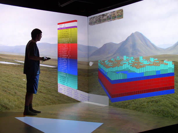
The use of WIT3D and ArcVeg combined calls for a three dimensional visualization to understand its dynamics. The data simulated is complex and components from individual models interact with each other. The choice was made to visualize the data in a three-dimensional virtual environment. It was recommended by the Arctic Region Supercomputing Center to use VR-Juggler. Cory Mohn, an ARSC summer intern, worked out the code for the original visualization tool. Data points are represented with cubes and the color of the cube represents a value interval. In the temperature setting, the color shades represent a temperature intervals, the scale is presented on the left side of the visualization. The user can chose to view ice accumulation through a color or through the height of the cubes. When the height of the cube is selected it is possible to view the temperature and the ice accumulation simultaneously. The Vegetation density on the soil surface is optional and is represented with a texture and the height of the vegetation cover cube. The textures are images of real vegetation in the field. The images were selected to represent a vegetation cover percentage. There are two ways to look inside the simulation domain. The first is to cut a section of cubes away from a corner. the second way of looking inside the solution domain is to make a color shade transparent. This results in three dimensional shapes and layers with the same color shade.